Formulation
This page summarizes the mathematical and numerical methods used by STEM to simulate railway-induced ground vibrations. STEM performs the numerical analysis of the train-track-soil system using the finite element method (FEM) and is powered by Kratos Multiphysics.
Governing equation
STEM solves the dynamic equilibrium equation, following a Total Lagrangian formulation with small strains. The governing finite element equation to be solved is:
\[\mathbf{M}\mathbf{a} + \mathbf{C}\mathbf{v} + \mathbf{K}\mathbf{u} = \mathbf{F_{ext}}\left( t \right)\]
where \(\mathbf{M}\) is the mass matrix, \(\mathbf{C}\) is the damping matrix, and \(\mathbf{K}\) is the stiffness matrix of the entire system, \(\mathbf{F_{ext}}\) denotes the vector of the external forces and \(\mathbf{a}\), \(\mathbf{v}\), \(\mathbf{u}\) are, respectively, the acceleration, the velocity and the displacement in the nodes.
In STEM it is also possible to perform quasi-static analyses, in which inertial and damping effects are neglected. In this case, the governing equation is reduced to:
\[\mathbf{K}\mathbf{u} = \mathbf{F_{ext}}\left( t \right).\]
Spatial discretisation
The spatial discretisation of the problem is performed using the finite element method (FEM). The geometry of the problem is built using gmsh and the mesh is generated and exported to Kratos mdpa format.
STEM supports several types of elements:
Beam elements (for 2D and 3D problems):
Euler-Bernoulli beam elements (2 nodes).
2D plane strain elements:
First order triangle elements (3 nodes per element)
Second order triangle elements (6 nodes per element)
3D solid elements:
First order tetrahedral elements (4 nodes per element)
Second order tetrahedral elements (10 nodes per element)
Time integration and solution strategies
The system of equations is solved in the time domain. A range of solution strategies are supported, including:
Implicit and explicit time integration schemes.
Nonlinear solution strategies (Newton-Raphson, line search, arc length).
For linear systems, it is recommended to use a custom explicit integration scheme based on the Newmark method, LinearNewtonRaphsonStrategy. This integration scheme takes advantage of the linear nature of the problem, and it is formulated explicitly. Following the Newmark method, the acceleration and velocity at time step \(n+1\) are calculated as:
where \(\Delta t\) is the time step for the numerical integration, the subscript \(\sqcup_{t + \Delta t}\) denotes kinematic variables at time \(t + \Delta t\), and \(\gamma\) and \(\beta\) are the parameters that control the integration accuracy and stability (the default values are \(\gamma = 0.5\) and \(\beta=0.25\)).
Substituting the Newmark equations into the governing equation, and taking advantage of the linearity of the problem, the system of equations yields:
where \(\mathbf{\widetilde{K}}\), \(\mathbf{\widetilde{a}}\) and \(\mathbf{\widetilde{v}}\) are the effective stiffness, acceleration and velocity, respectively, defined as:
The main advantage of using the custom Newmark explicit integration scheme is that it only requires once the assembly and factorisation of the entire system of matrices, making it computationally efficient for linear problems.
In STEM it is also possible to perform quasi-static analyses. In the quasi-static case, the governing equation is reduced to:
\[\mathbf{K}\mathbf{u} = \mathbf{F_{ext}}\left( t \right)\]
In this case, the system of equations is solved at each time step.
To solve the linear system of equations of type:
\[\mathbf{A}\mathbf{x} = \mathbf{b},\]
STEM has several linear solvers available, including:
LU decomposition
Conjugate Gradient
Algebraic Multigrid Iterative
The LU decomposition is a direct solver, which is suitable for small problems. The Conjugate Gradient and Algebraic Multigrid Iterative solvers are iterative solvers, which are suitable for large problems. The iterative solvers can use a preconditioner to improve the convergence rate, and they are recommended for large problems. In STEM the default preconditioner is the Jacobi preconditioner, which is a simple diagonal preconditioner that can be used for symmetric positive definite systems.
Boundary conditions
STEM support different types of boundary conditions, including:
Dirichlet boundary conditions (prescribed displacement or rotation)
Neumann boundary conditions (force or traction boundary conditions)
Absorbing boundary conditions [3]
Loads
STEM supports different types of loads, including:
Point, line, surface and moving loads
All the loads can be defined as time-dependent, and they can be applied to structural elements or soil.
For STEM it is important to be able to model the train-track interaction, which is the main source of the dynamic loading in the problem of railway-induced vibrations. To model the train-track interaction force STEM uses point moving loads, in combination with the UVEC (see Train-track model).
Constitutive models
STEM supports linear elastic material models. Non-linear material models can be implemented by the user and integrated into STEM through the UMAT API definition (see User-defined soil models).
Linear elastic material
STEM supports linear elastic material models. In STEM a material is defined by specifying the material formulation and the linear elastic material parameters.
Currently STEM supports the OnePhaseSoil material formulation. This formulation is used to model the soil as a single phase material, and it is defined by the following parameters:
Density of the solid phase \(\rho_s\)
Porosity \(n\)
Is_drained (boolean flag to indicate if the soil is drained or not)
The linear elastic material requires the following parameters for the OnePhaseSoil formulation:
Young’s modulus \(E\)
Poisson’s ratio \(\nu\)
In STEM the soil should be defined as OnePhaseSoil and the solution should be ‘drained’. This means that the soil is modelled as a single phase material and that the pore water pressure is not considered in the analysis. This is an assumption that is commonly used in the analysis of dynamic problems, such as railway-induced vibrations, and it is justified by the fact that the time scale of the problem is much shorter than the time scale of the pore water pressure dissipation.
Typically, the density of the bulk material is available from site investigations. The bulk density consists of the density of the solid phase and the density of the fluid phase, and it can be calculated as:
where \(\rho_f\) is the density of the fluid phase (water). Because in STEM the soil is modelled as a drained single phase material this equation simplifies to:
If the user has the bulk density and wants to use it as input, the porosity can be set to zero and the density of the solid phase can be set as the bulk density.
To model soil layers below ground water table, since the soil is modelled as a drained single phase material, the Poisson ratio of the soil layer should be set to 0.495. This means that the material is nearly incompressible, i.e. cannot experience volumetric deformation and this accurately mimics the saturated behaviour of soil, subjected to dynamic loading, in the short term (before pore water pressure dissipation occurs).
Interfaces
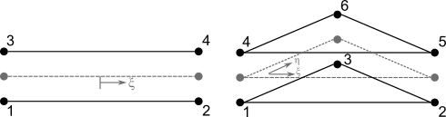
STEM supports the definition of interfaces between different soil or structural materials. An interface is represented as a zero-thickness layer whose mechanical response is governed by a constitutive law. The constitutive behaviour can be either linear elastic or non-linear. User-defined non-linear interface models can be implemented through the UMAT API definition (see User-defined soil models). For all interface constitutive laws, only the normal and tangential stiffness components are considered. This means that the interface element uses the \(\sigma_{zz}\), \(\sigma_{yz}\) and \(\sigma_{xz}\) from the stress tensor.
Interfaces can only be defined between lines, surfaces or volumes. Thus it cannot be defined between points.
The geometry is defined by two lines or planes, one on each side of the interface. The two sides of the interface connect to other model parts. Most calculations are performed on the ‘mid-geometry’, which is defined by the midpoints of the two lines/planes. The midpoints are calculated for each node pair by taking the average position. The mid-geometries are depicted as the grey lines in the figures below. This means, that if a certain property is queried at a certain position on the interface, the call is forwarded to the underlying mid-geometry.
Train-track model
The train and the train-track interaction model can be modelled by a user-defined vehicle model (UVEC) as described in User-defined vehicle model. STEM provides a default train and train-track interaction model.
Vehicle model
The train is modelled as a 2D mass-spring-damper system, with 10 degrees of freedom, that consists of a car body, bogies, suspension systems and wheels [6]. This model takes advantage of the system’s symmetry by simulating only half of the train, with symmetry boundary conditions applied to the central plane. The figure shows the schematic of the train model.
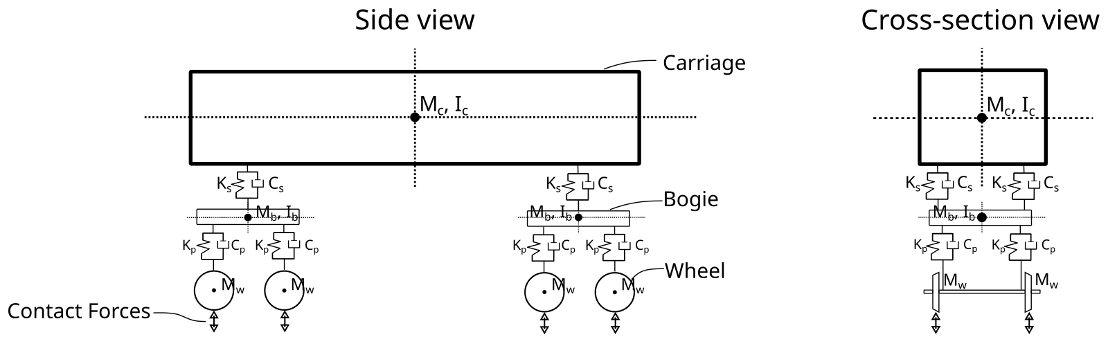
STEM train model
The railway track consists of rail, railpad and sleeper. The rail is modelled as an Euler-Bernoulli beam element. The railpad is modelled as a spring-damper element, which provides the stiffness and damping of the railpad. The sleeper can either be modelled as a concentrated mass, or a volume element, depending on the level of detail required by the user.
The parameters of the train and the train-track interaction model can be selected by the user from a range of predefined train types, or they can be defined by the user through the UVEC API definition. Please refer to UVEC load for more details on how to define the train and the train-track interaction model in STEM.
Interaction model
The vehicle and track systems are coupled through contact forces that occur at the interface between the wheels and the rails. These forces are determined using the non-linear Hertzian contact theory for metals [5]:
where \(k_\text{c}\) is the Hertzian stiffness coefficient and \(\delta_j\) is the vertical indentation between wheel \(j\) and the rail. If the indentation \(\delta_j\) is negative, the wheel is not in contact with the rail and the contact force is set to zero. The indentation \(\delta_j\) accounts for the relative wheel-rail displacement and the rail profile irregularity at the contact point:
where \(u_{\text{w},j}\) is the displacement of wheel \(j\), \(u_{\text{r},j}\) is the rail displacement at the contact location and \(r_j\) is the rail irregularity at the contact point. The total rail irregularity is represented as the sum of two components: the stochastic irregularity profile, \(r_w\), and the dipped joint irregularity, \(r_d\).
Irregularities model
The vertical rail irregularities (\(r_w\)) presented in the rail are expressed following the methodology presented in [7]. The power spectral density (PSD) of the rail irregularities \(S(\Omega)\) is used to produce the samples of the irregularities.
where \(\Omega\) the wavenumber, \(A_v\) the rail irregularity parameter and \(\Omega_c\) is the critical wavenumber. These two parameters define the quality of the railway track [2].
The sample of rail irregularities can be produced by inverse Fourier transform shown as follows:
where \(\Omega_n\), is the discrete wavenumber, \(\theta_n\), is a random phase angle uniformly distributed from 0 to \(2\pi\), and \(\Delta \Omega\) is the wavenumber increment.
The parameter \(A_v\) can be estimated based on the track quality [2].
Line grade |
Av Value (m² rad / m) |
|---|---|
1 (very poor) |
1.2107e-4 |
2 |
1.0181e-4 |
3 |
0.6816e-4 |
4 |
0.5376e-4 |
5 |
0.2095e-4 |
6 (very good) |
0.0339e-4 |
Rail joint model
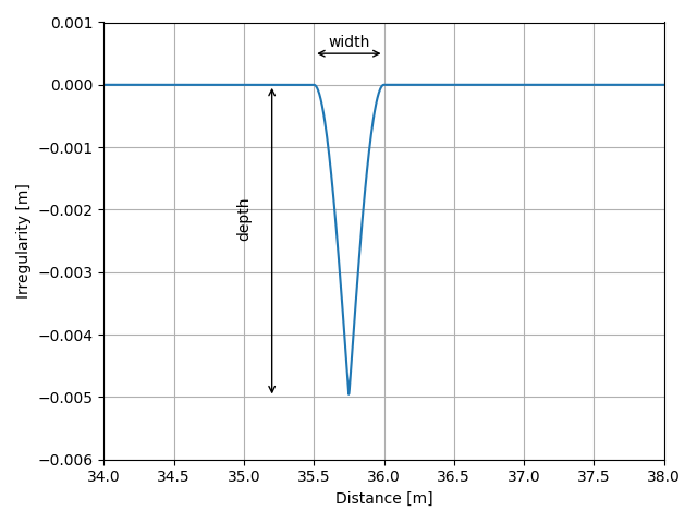
The rail joint is modelled as a hinge along a beam element, with a rotational stiffness defined based on the properties of the rail and the joint. The rail joint might have a local geometric irregularity, commonly referred to as a dipped joint, following the approach proposed by [1]. The dipped joint represents the permanent plastic deformation that develops at rail ends due to repeated wheel-rail impact loads at insulated joints.
The dip is introduced as a prescribed vertical rail surface irregularity with a smooth cosine shape, defined by its maximum depth \(d\) and total length \(l\). The vertical irregularity profile \(r_d(x)\) along the rail longitudinal coordinate \(x\) is given by:
where \(x = 0\) corresponds to the start of the dipped region. This formulation ensures a continuous and smooth rail profile with zero slope at the beginning and end of the joint, avoiding artificial high-frequency excitation.
A schematic of the dipped joint is shown in the figure below.
Schematic of the dipped joint model