Lamb’s problem in 3D
Overview
This tutorial shows how to set up and run a 3D Lamb problem. The Lamb problem consists of the application of a point load on the surface of an elastic half-space, and computing the wave propagation towards the free field. To avoid reflections at the model edges, absorbing boundary conditions are used.
Imports and setup
First the necessary packages are imported and the input folder is defined.
input_files_dir = "lamb"

from stem.model import Model
from stem.soil_material import OnePhaseSoil, LinearElasticSoil, SoilMaterial, SaturatedBelowPhreaticLevelLaw
from stem.load import PointLoad
from stem.boundary import DisplacementConstraint, AbsorbingBoundary
from stem.solver import AnalysisType, SolutionType, TimeIntegration, DisplacementConvergenceCriteria, \
    StressInitialisationType, SolverSettings, Problem, LinearNewtonRaphsonStrategy, Cg
from stem.output import NodalOutput, VtkOutputParameters, JsonOutputParameters
from stem.stem import Stem
For setting up the model, Model is imported from stem.model.
For the soil material, OnePhaseSoil, LinearElasticSoil, SoilMaterial,
and SaturatedBelowPhreaticLevelLaw are imported from stem.soil_material.
In this case, a point load is applied, therefore PointLoad is imported from stem.load.
Boundary conditions are set using DisplacementConstraint and AbsorbingBoundary.
Solver settings are defined with classes imported from stem.solver.
For output, NodalOutput, VtkOutputParameters, and JsonOutputParameters are imported.
Finally, Stem is imported from stem.stem to write input files and run the calculation.
Geometry and materials
In this step, the geometry and materials are defined. First the model dimension is set to 3 and the model is initialised.
ndim = 3
model = Model(ndim)
The soil is modelled as linear-elastic, drained, and one-phase material. The material parameters are defined as follows.
DENSITY_SOLID = 2000
POROSITY = 0
YOUNG_MODULUS = 30e6
POISSON_RATIO = 0.2

soil_formulation = OnePhaseSoil(ndim, IS_DRAINED=True, DENSITY_SOLID=DENSITY_SOLID, POROSITY=POROSITY)
constitutive_law = LinearElasticSoil(YOUNG_MODULUS=YOUNG_MODULUS, POISSON_RATIO=POISSON_RATIO)
retention_parameters = SaturatedBelowPhreaticLevelLaw()
material = SoilMaterial("soil", soil_formulation, constitutive_law, retention_parameters)
A rectangular soil domain is created in the x-y plane and extruded in z-direction. The layer coordinates are defined and the soil layer is added to the model.
x_max = 10
y_max = 5
z_max = 10

layer_coordinates = [(0.0, 0.0, 0.0), (x_max, 0.0, 0.0), (x_max, y_max, 0.0), (0.0, y_max, 0.0)]
model.extrusion_length = z_max

model.add_soil_layer_by_coordinates(layer_coordinates, material, "soil")
Load
A point load is applied at the surface corner (x=0, y=y_max, z=0), acting in the negative y-direction. The load is suddenly applied with an amplitude of \(10^6\) N.
force = -1e6
node_coordinates = [(0.0, y_max, 0.0)]

point_load = PointLoad(active=[True, True, True], value=[0, force, 0])
model.add_load_by_coordinates(node_coordinates, point_load, "point_load")
Boundary conditions
Below the boundary conditions are defined. The bottom base is fully fixed in all directions. Roller boundaries are applied on x=0 and z=0 planes. Absorbing boundary conditions are applied on x=x_max and z=z_max planes.
no_displacement_parameters = DisplacementConstraint(is_fixed=[True, True, True],
                                                    value=[0, 0, 0])
roller_displacement_parameters_x = DisplacementConstraint(is_fixed=[True, False, False],
                                                          value=[0, 0, 0])
roller_displacement_parameters_z = DisplacementConstraint(is_fixed=[False, False, True],
                                                          value=[0, 0, 0])
abs_boundary_parameters = AbsorbingBoundary(absorbing_factors=[1.0, 1.0], virtual_thickness=10)

model.add_boundary_condition_on_plane([(0, 0, 0), (x_max, 0, 0), (x_max, 0, z_max)], no_displacement_parameters,
                                      "base_fixed")
model.add_boundary_condition_on_plane([(0, 0, 0), (0, y_max, 0), (0, y_max, z_max)],
                                      roller_displacement_parameters_x, "sides_roler_x=0")
model.add_boundary_condition_on_plane([(0, 0, 0), (x_max, 0, 0), (x_max, y_max, 0)],
                                      roller_displacement_parameters_z, "sides_roler_z=0")
model.add_boundary_condition_on_plane([(x_max, 0, 0), (x_max, y_max, 0), (x_max, y_max, z_max)],
                                      abs_boundary_parameters, "abs_x=x_max")
model.add_boundary_condition_on_plane([(0, 0, z_max), (x_max, 0, z_max), (x_max, y_max, z_max)],
                                      abs_boundary_parameters, "abs_z=z_max")
Mesh
The mesh size and element order are defined. After assigning geometry and conditions, the geometry is synchronised.
model.set_mesh_size(element_size=1)
model.mesh_settings.element_order = 2

model.synchronise_geometry()
Solver settings
Now that the model is defined, the solver settings should be set.
The analysis type is set to MECHANICAL and the solution type to DYNAMIC. The start time is set to 0.0 s and the end time is set to 0.08 s. The time step for the analysis is set to 0.01 s. The system of equations is solved with the assumption of constant stiffness matrix, mass matrix, and damping matrix. The Linear-Newton-Raphson (Newmark explicit solver) is used as strategy and Cg as solver for the linear system of equations.
The Rayleigh damping parameters are set to \(\alpha = 0.248\) and \(\beta = 7.86 \cdot 10^{-5}\), which correspond to a damping ratio of 2% for 1 and 80 Hz.
The convergence criterion for the numerical solver are set to a relative tolerance of \(10^{-4}\) and an absolute tolerance of \(10^{-9}\) for the displacements.
time_step = 0.01

time_integration = TimeIntegration(start_time=0.0,
                                   end_time=0.08,
                                   delta_time=time_step,
                                   reduction_factor=1.0,
                                   increase_factor=1.0,
                                   max_delta_time_factor=1000)

convergence_criterion = DisplacementConvergenceCriteria(displacement_relative_tolerance=1.0e-4,
                                                        displacement_absolute_tolerance=1.0e-9)

solver_settings = SolverSettings(analysis_type=AnalysisType.MECHANICAL,
                                 solution_type=SolutionType.DYNAMIC,
                                 stress_initialisation_type=StressInitialisationType.NONE,
                                 time_integration=time_integration,
                                 is_stiffness_matrix_constant=True,
                                 are_mass_and_damping_constant=True,
                                 convergence_criteria=convergence_criterion,
                                 strategy_type=LinearNewtonRaphsonStrategy(),
                                 linear_solver_settings=Cg(),
                                 rayleigh_k=7.86e-5,
                                 rayleigh_m=0.248)
Problem and output
The problem definition is added to the model. The problem name is set to “Lamb”, the number of threads is set to 8 and the solver settings are applied.
In this example, JSON output is requested at 2 surface points (displacements) and VTK output is written for the full computational model part (displacements and velocities).
problem = Problem(problem_name="Lamb", number_of_threads=8, settings=solver_settings)
model.project_parameters = problem
json_output_parameters = JsonOutputParameters(time_step, [NodalOutput.DISPLACEMENT], [])
model.add_output_settings_by_coordinates([
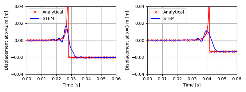
(2, y_max, 0),
(3, y_max, 0),
], json_output_parameters, "json_output")
model.add_output_settings(
output_parameters=VtkOutputParameters(
file_format="ascii",
output_interval=1,
nodal_results=[NodalOutput.DISPLACEMENT, NodalOutput.VELOCITY],
gauss_point_results=[],
output_control_type="step"
),
part_name="porous_computational_model_part",
output_dir="output",
output_name="vtk_output"
)
Run
Now that the model is set up, the calculation is ready to run.
Firstly the Stem class is initialised, with the model and the directory where the input files will be written to.
While initialising the Stem class, the mesh will be generated.
This is followed by writing all the input files required to run the calculation.
The calculation is run by calling stem.run_calculation().
stem = Stem(model, input_files_dir)
stem.write_all_input_files()
stem.run_calculation()
Results
Once the calculation is finished, the results can be visualised using Paraview, or by loading the JSON output file.
This figure shows the time history of the vertical displacements at the two points along the surface (these results have been obtained for a time step of 0.001 s, time duration of 0.15 s and with an element size of 0.25 m, and are different from the ones presented in the tutorial above). The results are compared with the analytical solution of the Lamb problem.
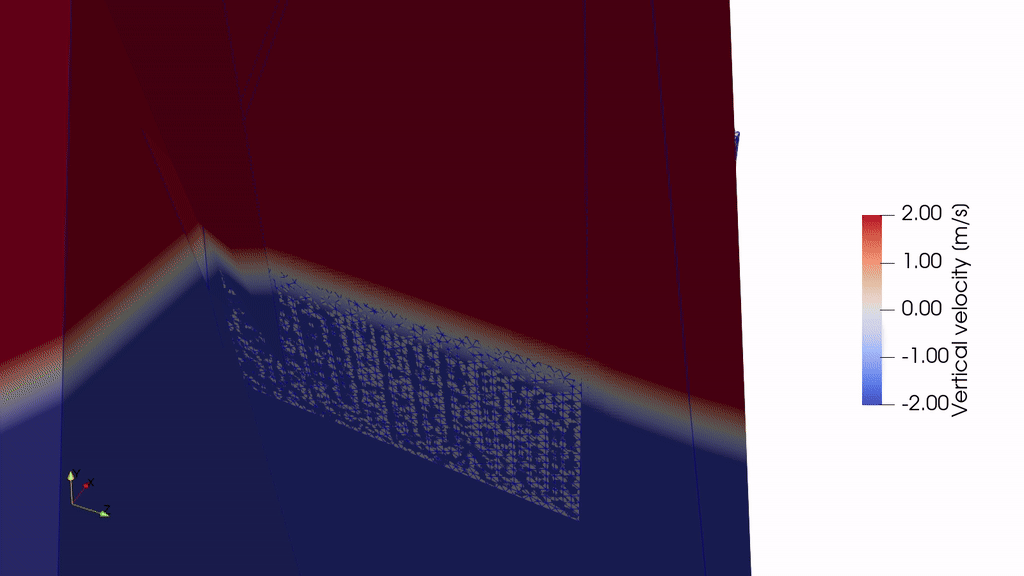
This animation shows the vertical velocity of the soil when subjected to the pulse load.
See also