Moving load on an embankment in 3D
Overview
This tutorial shows how to set up a moving load on top of an embankment with two soil layers underneath, in a 3D model. The moving load is applied on top of the embankment and moves in the z-direction at constant velocity.
Imports and setup
First the necessary packages are imported and the input folder is defined.
input_files_dir = "moving_load"

from stem.model import Model
from stem.soil_material import OnePhaseSoil, LinearElasticSoil, SoilMaterial, SaturatedBelowPhreaticLevelLaw
from stem.load import MovingLoad
from stem.boundary import DisplacementConstraint
from stem.solver import AnalysisType, SolutionType, TimeIntegration, DisplacementConvergenceCriteria,\
        LinearNewtonRaphsonStrategy, NewmarkScheme, Cg, StressInitialisationType, SolverSettings, Problem
from stem.output import NodalOutput, VtkOutputParameters, JsonOutputParameters
from stem.stem import Stem
For setting up the model, Model is imported from stem.model.
For the soil material, OnePhaseSoil, LinearElasticSoil, SoilMaterial,
and SaturatedBelowPhreaticLevelLaw are imported from stem.soil_material.
In this case, a moving load is applied, therefore MovingLoad is imported from stem.load.
Boundary conditions are set using DisplacementConstraint.
Solver settings are defined with classes imported from stem.solver.
For output, NodalOutput and VtkOutputParameters are imported.
Finally, Stem is imported from stem.stem to write input files and run the calculation.
Geometry and materials
In this step, the geometry, and material parameters for the simulation are defined. First the dimension of the model is indicated which in this case is 3. After which the model can be initialised.
ndim = 3
model = Model(ndim)
Specification of the soil material is defined afterwards. The bottom soil layer is defined as a material with the name “soil_1”. It is a Linear elastic material model with the solid density of 2650 kg/m3, the Young’s modulus is 30e6 Pa and the Poisson’s ratio is of 0.2. A porosity of of 0.3 is specified. The soil is a one-phase soil, meaning that the flow of water through the soil is not computed.
solid_density_1 = 2650
porosity_1 = 0.3
young_modulus_1 = 30e6
poisson_ratio_1 = 0.2
soil_formulation_1 = OnePhaseSoil(ndim, IS_DRAINED=True, DENSITY_SOLID=solid_density_1, POROSITY=porosity_1)
constitutive_law_1 = LinearElasticSoil(YOUNG_MODULUS=young_modulus_1, POISSON_RATIO=poisson_ratio_1)
retention_parameters_1 = SaturatedBelowPhreaticLevelLaw()
material_soil_1 = SoilMaterial("soil_1", soil_formulation_1, constitutive_law_1, retention_parameters_1)
The second soil layer is defined as a material with the name “soil_2”. It is a Linear elastic material model with the solid density of 2550 kg/m3, the Young’s modulus is 30e6 Pa and the Poisson’s ratio is 0.2. A porosity of 0.3 is specified. The soil is a one-phase soil, meaning that the flow of water through the soil is not computed.
solid_density_2 = 2550
porosity_2 = 0.3
young_modulus_2 = 30e6
poisson_ratio_2 = 0.2
soil_formulation_2 = OnePhaseSoil(ndim, IS_DRAINED=True, DENSITY_SOLID=solid_density_2, POROSITY=porosity_2)
constitutive_law_2 = LinearElasticSoil(YOUNG_MODULUS=young_modulus_2, POISSON_RATIO=poisson_ratio_2)
retention_parameters_2 = SaturatedBelowPhreaticLevelLaw()
material_soil_2 = SoilMaterial("soil_2", soil_formulation_2, constitutive_law_2, retention_parameters_2)
The embankment layer on top is defined as a material with the name “embankment”. It is a Linear elastic material model with the solid density of 2650 kg/m3, the Young’s modulus is 10e6 Pa and the Poisson’s ratio is 0.2. A porosity of 0.3 is specified. The soil is a one-phase soil, meaning that the flow of water through the soil is not computed.
solid_density_3 = 2650
porosity_3 = 0.3
young_modulus_3 = 10e6
poisson_ratio_3 = 0.2
soil_formulation_3 = OnePhaseSoil(ndim, IS_DRAINED=True, DENSITY_SOLID=solid_density_3, POROSITY=porosity_3)
constitutive_law_3 = LinearElasticSoil(YOUNG_MODULUS=young_modulus_3, POISSON_RATIO=poisson_ratio_3)
retention_parameters_3 = SaturatedBelowPhreaticLevelLaw()
material_embankment = SoilMaterial("embankment", soil_formulation_3, constitutive_law_3, retention_parameters_3)
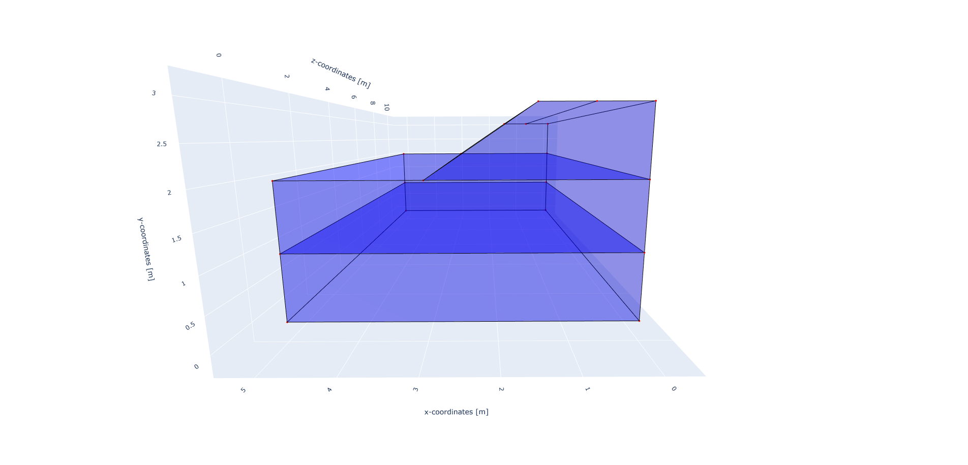
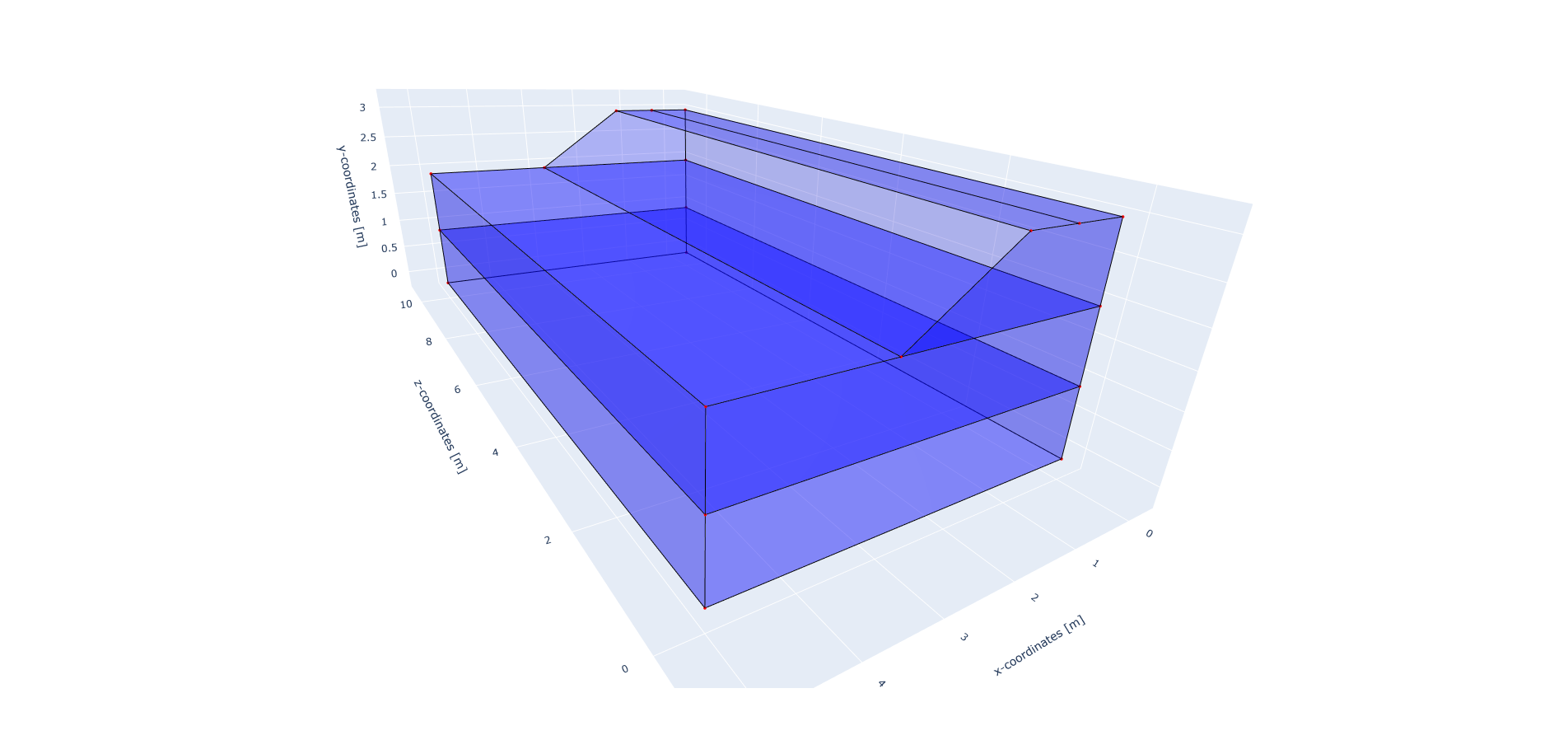
The geometry of the model is defined afterwards. The model consists of two soil layers and an embankment on top. Each layer is defined by a list of coordinates, defined in the x-y plane. The coordinates are defined in clockwise or anti-clockwise order, and the first and last coordinates are not the same, since the geometry will be closed. To generate a full 3D model, the geometry in the x-y plane is extruded in the z-direction. In this case, the extrusion length is 50 m.
soil1_coordinates = [(0.0, 0.0, 0.0), (5.0, 0.0, 0.0), (5.0, 1.0, 0.0), (0.0, 1.0, 0.0)]
soil2_coordinates = [(0.0, 1.0, 0.0), (5.0, 1.0, 0.0), (5.0, 2.0, 0.0), (0.0, 2.0, 0.0)]
embankment_coordinates = [(0.0, 2.0, 0.0), (3.0, 2.0, 0.0), (1.5, 3.0, 0.0), (0.75, 3.0, 0.0), (0, 3.0, 0.0)]
model.extrusion_length = 50
The geometry is shown in the figures below.
The soil layers are then added to the model in the following way. It is important that all soil layers have a unique name.
model.add_soil_layer_by_coordinates(soil1_coordinates, material_soil_1, "soil_layer_1")
model.add_soil_layer_by_coordinates(soil2_coordinates, material_soil_2, "soil_layer_2")
model.add_soil_layer_by_coordinates(embankment_coordinates, material_embankment, "embankment_layer")
Load
The moving load is modelled using the MovingLoad class.
The load is defined following a list of coordinates.
In this case, a moving load is applied along a line located at 0.75 m distance from the x-axis on top of the embankment.
The velocity of the moving load is 30 m/s and the load is -10000 N in the y-direction.
The load moves in positive z-direction and the load starts at coordinates: [0.75, 3.0, 0.0].
It is possible to use different types of loads. Please refer to Loads for more information on the different load types and how to define them.
load_coordinates = [(0.75, 3.0, 0.0), (0.75, 3.0, 50.0)]
moving_load = MovingLoad(load=[0.0, -10000.0, 0.0], direction_signs=[1, 1, 1], velocity=30, origin=[0.75, 3.0, 0.0],
                         offset=0.0)
model.add_load_by_coordinates(load_coordinates, moving_load, "moving_load")
Boundary conditions
Below the boundary conditions are defined. The base of the model is fixed in all directions with the name “base_fixed”. The roller boundary condition is applied on the sides of the embankment with the name “sides_roller”. The boundary conditions are applied on plane surfaces defined by a list of coordinates.
no_displacement_parameters = DisplacementConstraint(is_fixed=[True, True, True], value=[0, 0, 0])
roller_displacement_parameters = DisplacementConstraint(is_fixed=[True, False, True], value=[0, 0, 0])

model.add_boundary_condition_on_plane([(0.0, 0.0, 0.0), (5.0, 0.0, 0.0), (5.0, 0.0, 50)], no_displacement_parameters,
                                      "base_fixed")
model.add_boundary_condition_on_plane([(0, 0, 0), (0, 3, 0), (0, 3, 50)],
                                      roller_displacement_parameters, "sides_roler_x=0")
model.add_boundary_condition_on_plane([(0, 0, 0), (5, 0, 0), (5, 3, 0)],
                                      roller_displacement_parameters, "sides_roler_z=0")
model.add_boundary_condition_on_plane([(5, 0, 0), (5, 3, 0), (5, 3, 50)],
                                      roller_displacement_parameters, "sides_roler_x=5")
model.add_boundary_condition_on_plane([(0, 0, 50), (5, 0, 50), (5, 1, 50)],
                                      roller_displacement_parameters, "sides_roler_z=50")
Alternatively, the boundary conditions can also be added by geometry IDs.
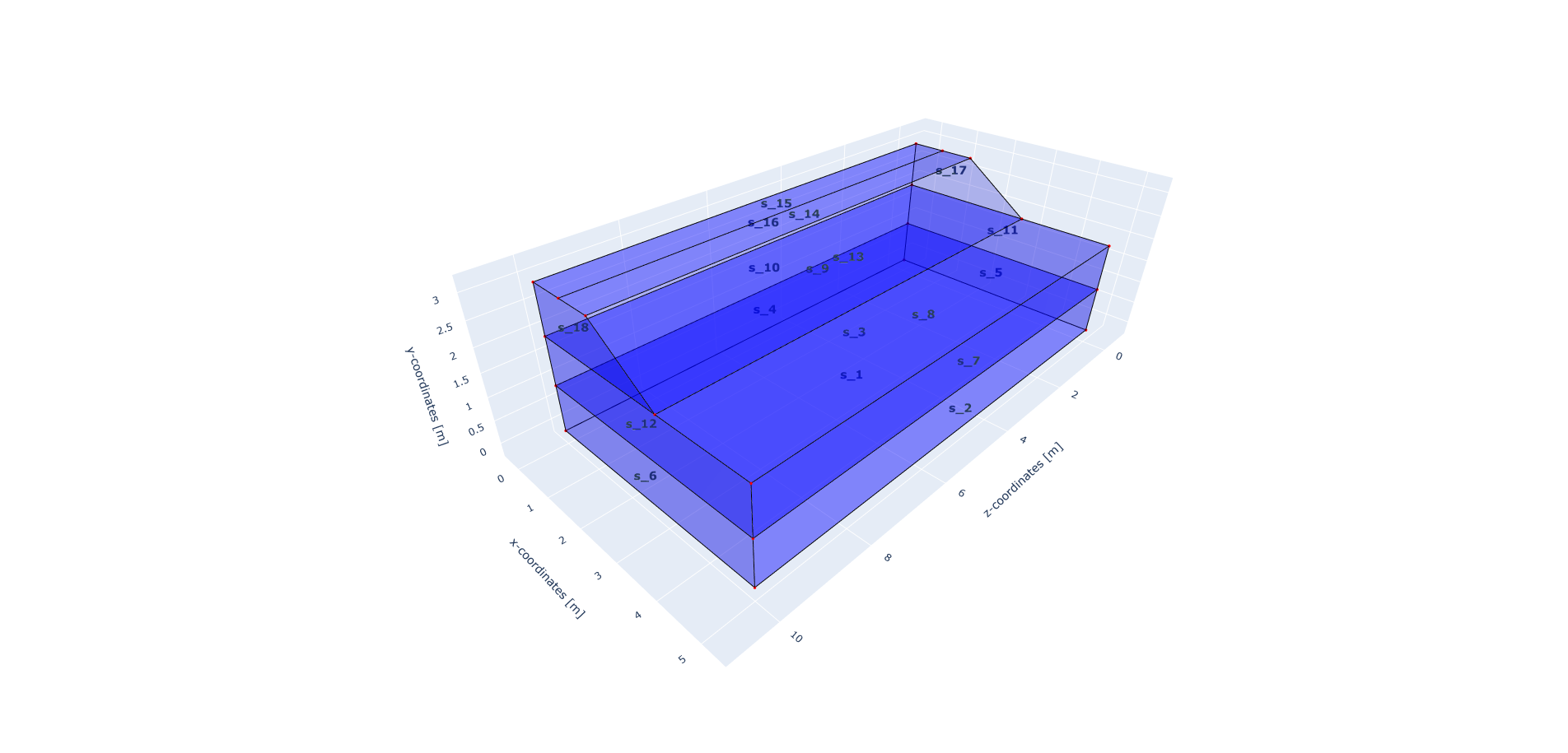
The roller boundary condition is active in the y-direction, meaning that the boundary conditions are added to the model on the edge surfaces, i.e. the boundary conditions are applied to a list of surface IDs (which can be visualised using: “model.show_geometry(show_surface_ids=True)”) with the corresponding dimension, “2”.
no_displacement_parameters = DisplacementConstraint(is_fixed=[True, True, True], value=[0, 0, 0])
roller_displacement_parameters = DisplacementConstraint(is_fixed=[True, False, True], value=[0, 0, 0])

model.add_boundary_condition_by_geometry_ids(2, [1], no_displacement_parameters, "base_fixed")
model.add_boundary_condition_by_geometry_ids(2, [2, 4, 5, 6, 7, 10, 11, 12, 16, 17, 18],
                                             roller_displacement_parameters, "sides_roller")
To inspect the geometry IDs, the geometry can be visualised using the model.show_geometry function.
This function can be used for visualisation of the geometry IDs after creation of the geometry, so that it is known
which ID belong to each boundary condition.
For visualisation of surface IDs, show_surface_ids should be set to True.
Also for visualisation of line IDs, show_line_ids and for visualisation of point IDs, show_point_ids
should be set to True.
model.synchronise_geometry()

model.show_geometry(show_surface_ids=True)
The geometry IDs can be seen in the pictures below.
Mesh
The mesh size and element order are defined. The element size for the mesh can be defined as a single value, which will be applied to the whole model.
model.set_mesh_size(element_size=1.0)
model.mesh_settings.element_order = 1
Alternatively, the element size can also be defined for each soil layer separately:
model.set_mesh_size(element_size=1.0)
model.set_element_size_of_group(0.5, "soil_layer_1")
model.set_element_size_of_group(1.5, "soil_layer_2")
model.set_element_size_of_group(1, "embankment_layer")
Solver settings
Now that the model is defined, the solver settings should be set.
The analysis type is set to MECHANICAL and the solution type to DYNAMIC. The start time is set to 0.0 s and the end time is set to 1.5 s. The time step for the analysis is set to 0.01 s. The system of equations is solved with the assumption of constant stiffness matrix, mass matrix, and damping matrix. The Linear-Newton-Raphson (Newmark explicit solver) is used as strategy and Cg as solver for the linear system of equations.
The Rayleigh damping parameters are set to \(\alpha = 0.248\) and \(\beta = 7.86 \cdot 10^{-5}\), which correspond to a damping ratio of 2% for 1 and 80 Hz.
The convergence criterion for the numerical solver are set to a relative tolerance of \(10^{-4}\) and an absolute tolerance of \(10^{-9}\) for the displacements.
# Set up start and end time of calculation, time step
time_integration = TimeIntegration(start_time=0.0, end_time=1.5, delta_time=0.01, reduction_factor=1.0,
                                   increase_factor=1.0)
convergence_criterion = DisplacementConvergenceCriteria(displacement_relative_tolerance=1.0e-4,
                                                        displacement_absolute_tolerance=1.0e-9)

solver_settings = SolverSettings(analysis_type=AnalysisType.MECHANICAL,
                                 solution_type=SolutionType.DYNAMIC,
                                 stress_initialisation_type=StressInitialisationType.NONE,
                                 time_integration=time_integration,
                                 is_stiffness_matrix_constant=True,
                                 are_mass_and_damping_constant=True,
                                 convergence_criteria=convergence_criterion,
                                 strategy_type=LinearNewtonRaphsonStrategy(),
                                 linear_solver_settings=Cg(),
                                 rayleigh_k=7.86e-5,
                                 rayleigh_m=0.248)
Problem and output
The problem definition is added to the model. The problem name is set to “moving_load_on_embankment_3d”, the number of threads is set to 8 and the solver settings are applied.
problem = Problem(problem_name="moving_load_on_embankment_3d", number_of_threads=8,
                  settings=solver_settings)
model.project_parameters = problem
Before starting the calculation, it is required to specify the desired output. In this case, displacement, and velocity are requested on the nodes and written into VTK files. Gauss point results (stresses) are left empty.
The JSON output file is requested at a point located in the surface of the embankment, in the middle of the model, with coordinates (0.75, 3.0, 25.0).
The output process is added to the model using the Model.add_output_settings method.
The results are written to the output directory in VTK format.
In this case, the output interval is set to 1 and the output control type is set to step, meaning that the
results will be written every time step.
json_output_parameters = JsonOutputParameters(0.01, [NodalOutput.DISPLACEMENT], [])

model.add_output_settings_by_coordinates([
    (0.75, 3.0, 25.0)],
    json_output_parameters,
    "json_output")

nodal_results = [NodalOutput.DISPLACEMENT, NodalOutput.VELOCITY]
gauss_point_results = []

model.add_output_settings(
    part_name="porous_computational_model_part",
    output_name="vtk_output",
    output_dir="output",
    output_parameters=VtkOutputParameters(
        output_interval=1,
        nodal_results=nodal_results,
        gauss_point_results=gauss_point_results,
        output_control_type="step"
    )
)
Run
Now that the model is set up, the calculation is ready to run.
Firstly the Stem class is initialised, with the model and the directory where the input files will be written to.
While initialising the Stem class, the mesh will be generated.
This is followed by writing all the input files required to run the calculation.
The calculation is run by calling stem.run_calculation().
stem = Stem(model, input_files_dir)
stem.write_all_input_files()
stem.run_calculation()
Results
Once the calculation is finished, the results can be visualised using Paraview, or by loading the JSON output file.
This figure shows the time history of the vertical displacements at the point on the embankment surface (these results have been obtained for a time step of 0.005 s, time duration of 1.75 s and with an element size of 0.5 m).
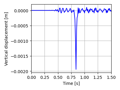
This animation shows the vertical displacement of the soil due to the moving load.
See also
Previous: Lamb’s problem in 3D
Next: Embankment over bridge